

1. Introduction
2. Experimental Apparatus for Investigating Hydrogen-CO2-Air Tubular Flame with Raman Scattering Technique
2.1 Tubular burner
2.2 Raman scattering system
3. Calibration of Raman Signal
4. A Hydrogen-CO2-Air Partially Premixed Cellular Tubular Flame
5. Conclusion
1. Introduction
Raman scattering phenomenon was first discovered by Raman in 1928 [1]. However, it was not applied to flame measurement until the advent of laser in the 1970s. Since the pioneering investigations of Lapp and Penney [2, 3], spontaneous Raman scattering technique has been received much attention for combustion diagnostics. In their work, the first spontaneous Raman scattering measurements in flames were made using a continuous wave (CW) argon ion (Ar+) laser to measure the vibrational Raman scattering spectra of H2O, N2, and O2 in flames where the flame temperature was interpreted from spectral fits. Since then, the technique has been widely applied to measure major species concentrations and temperature in various flames, for example, in planar opposed-jet flames [4, 5], premixed tubular flames [6, 7], and nonpremixed opposed-flow tubular flames [8, 9]. There are excellent reviews of Raman scattering technique, in terms of theory and measurement in flames [3, 10, 11, 12].
The theoretical background for Raman scattering is complex and the detailed description is left to other references [11, 13]. A brief description follows, nonetheless. As a laser beam passes through a flame, light is scattered from molecules of the flame both elastically (Rayleigh scattering) and inelastically (Raman scattering). Fig. 1 shows energy diagram of both Rayleigh and Raman scattering processes of a diatomic molecule and their corresponding spectra. Rayleigh scattered light, which is about 1,000 times stronger than Raman counterpart, is shifted slightly by the gas velocity and its spectrum can be used to measure temperature, density, and velocity [14, 15]. In the Raman process, light scattered from rotating and vibrating molecules is shifted by a change in the rotational and/or vibrational energy level of the molecule. Rotational energy changes are small and pure rotational Raman scattering lies close to the exciting laser wavelength. For vibrational Raman scattering, the Q branch gives the strongest spectral line with selection rules for the vibrational quantum number ν of △ν=±1. Vibrational energy changes are much larger leading to vibrational Raman lines that are far from the exciting laser line. In vibrational Stokes Raman scattering, the molecule absorbs some of the incident photon energy leading to a red-shifted photon, while the scattered photon in anti-Stokes Raman scattering is blue-shifted. Since Stokes scattering is much stronger than anti-Stokes one, the former is used in flame measurements.
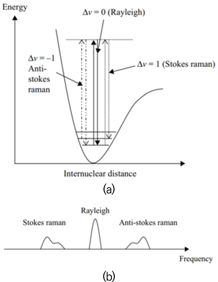
Fig. 1.
Vibrational Raman and Rayleigh scattering processes: (a) energy diagram of a diatomic molecule and (b) their light spectrum [17].
The Raman signals contain a signature of the molecular content of the gas mixture; this allows the use of a single laser source to characterize the entire content of the gas mixture. The compromise of using spontaneous Raman scattering for gas phase measurements is that the signals are relatively weak, and only the major chemical species can be detected. Vibrational Raman shifts and their corresponding Stokes wavelength for a 532 nm Nd:YAG laser are given in Table 1 for combustion species commonly measured in flames. The Raman shifts of other molecules are published elsewhere [11, 16].
Table 1.
Frequency-shifts and related emission wavelengths with the excitation of 532 nm Nd:YAG laser for various species formed in flames [17]
| Species | Frequency shift (cm-1) | Wavelength (nm) |
| CO2 | 1285, 1388 | 571.0, 574.4 |
| O2 | 1556 | 580.0 |
| CO | 2145 | 600.5 |
| N2 | 2330.7 | 607.3 |
| CH4 | 2915, 3017 | 629.6, 633.7 |
| H2O | 3657 | 660.5 |
| H2 | 4160 | 683.2 |
The processing of Raman scattering signals into concentrations needs to account for the temperature dependence of Raman spectra. Also, Raman spectra of certain species overlap: for example, there is cross-talk between CO2 and O2. In addition, there can be interferences from laser induced fluorescence and from broad-band flame luminosity [18, 19]. There have been two different approaches to Raman data processing: the spectral fitting (SF) method [20, 21], based on libraries of theoretical spectra; and the matrix inversion (MI) method [22, 23], based on extensive calibration of temperature-dependent system response. Each method has advantages and disadvantages. The MI method allows for lower readout noise due to on-chip binning, and processing is fast. However, extensive calibration is needed, and uncertainties in calibrations of reactive species and cross-talk terms at flame temperatures can be large. On the other hand, the SF method reduces the number of calibrations to only one per species and reduces uncertainty within temperature ranges that are difficult to calibrate. However, the preserved spectral information comes with the price of higher readout noise, slower data acquisition rates, and significant effort fitting the Raman spectrum of each single-shot measurement [24]. There is also a hybrid approach combining the advantages of both methods [24].
The number of detected photons for a Q-branch line for ith chemical species can estimated by,
where EL is the laser energy, σzz is the vibrational Raman cross section, Xi is the species mole fraction, N is the total number density, L is the spatial resolution along the laser beam, Ω is the collection solid angle, η is the efficiency of the detection system, Qe is the quantum efficiency of the back-illuminated CCD camera, Γ(T) is the temperature- dependent factor that accounts for the distribution of the molecules among the vibrational states, λ is the Stokes Raman wavelength, h is Planck’s constant, and c is the speed of light.
In the MI method, quantitative number densities of the major species Nj (#/cc) can be determined from the simplified form of Eq. (1) as below:
where Si is the Raman signal, E is the total integrated laser pulse energy, f is the experimentally derived spatially dependent attenuation factor, and Kij is the temperature dependent calibration coefficient matrix, indicating the degree of contribution of Raman signal of jth species on to that of ith species. The calibration coefficient matrix can be determined by making Raman measurements in the near adiabatic equilibrium region of a flame from a Hencken burner [25], which has very little heat loss at a high flow rate. Then an adiabatic equilibrium program (e.g., Cantera [26]) can be used to calculate the composition and temperature in the region. Usually, the temperature dependent calibration matrices are determined from 300 K to 2200 K for the most of flames studied [17]. It is noted that this form is valid for a fixed detection setup; a more complete formulation is discussed elsewhere [11, 22]. Also, the gas temperature can be given by,
where p0 is the thermodynamic pressure (Pa) and kb is the Boltzmann’s constant (1.38 × 10⁻²³ J/K).
In this paper, the technical approach including data reduction of the Raman scattering technique for measurements of major species (CO2, O2, N2, H2O, and H2) concentrations and temperature in tubular flames, from experimentally collecting the Raman spectra to reducing the experimental data for the measurements, is described. Raman scattering data for investigating the structure of hydrogen-CO2-air partially-premixed cellular tubular flames [27] have been borrowed for this study. Existing MATLAB scripts for preparing for the experiments, calibrating Raman signals, reducing Raman spectra, and finally plotting the results have been reviewed and modified, as needed. The approach described here for hydrogen/air tubular flame may be extended to hydrocarbon/air tubular flames when other necessary major species, for example, CH4 and CO for methane/air tubular flame, are considered in the experiment and data reduction processes.
2. Experimental Apparatus for Investigating Hydrogen-CO2-Air Tubular Flame with Raman Scattering Technique
To better understand the data reduction procedures for Raman scattering technique to be explained at the following chapters, the experimental apparatus including a uniquely designed tubular burner and Raman spectroscopy system at Vanderbilt University [27] are briefly explained here. More detailed descriptions of the system are found elsewhere [27].
2.1 Tubular burner
A uniquely designed tubular burner was developed − premixed [7], non-premixed or diffusion [9], and partially- premixed [27] − to lower the complexity of the combustion process from a turbulent, transient, three-dimensional problem to a laminar, steady-state, two-dimensional and/or one-dimensional one. As shown in Fig. 2, the tubular burner produces a radially-opposed flow field where the fluid stagnates about an axial coordinate in the shape of either a cylindrical face or a line, unlike the traditional flow field created by opposed-axial jets where the fluid stagnates about a plane. The configuration stagnating about a line, shown in Fig. 2 (RHS), has a single inlet, the outer nozzle, and can be used for premixed studies while the one stagnating to a cylindrical surface by adding an inner nozzle, in the center figure, can be used for studying pure diffusion and partially-premixed flames (PPF).
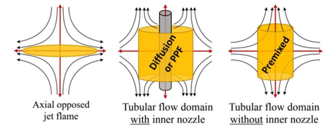
Fig. 2.
Flowfields for an axial-opposed jet flame (LHS), radially-opposed jet flames with two nozzles (CTR) and a single nozzle (RHS) [28].
Detailed axisymmetric view of PPF tubular burner is shown in Fig. 3. The premixed combustible gases are introduced from the outer chamber, and impinge against as opposing diluted fuel flow from a porous inner nozzle, resulting in a cylindrical stagnation surface with axial divergence, which creates PPF. For creating premixed flames with all reactants exiting the outer nozzle, the reacting flow domain is a 24 mm diameter with an 8 mm nozzle height with non-reacting co-flow nozzles to preserve uniform inlet velocities and temperature. Addition of a porous pipe, an inner nozzle, modifies the flow domain and permits formation of tubular diffusion flames with the oxidizer exiting the outer nozzle and fuel exiting the inner nozzle. The inner nozzle is 6.2 mm in diameter and has an 8 mm section in height for fuel with the remainder of the nozzle designed as a co-flow. For PPF, lean premixed gases are introduced by the outer annular nozzle and diluted fuels exit the porous inner nozzle.
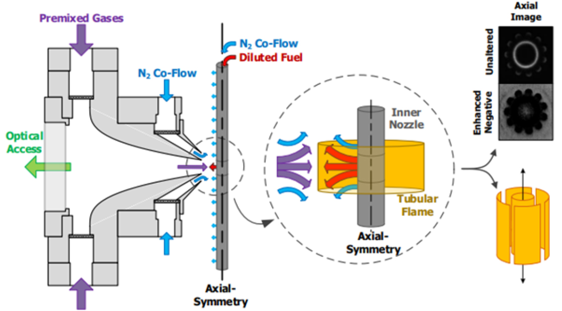
Fig. 3.
Axisymmetric view of the PPF tubular burner and formation of n-fold cellular tubular flame [27].
The stagnation surface radius and the stretch rate (κ) are functions of radial velocities, mixture density, and the nozzle radii [29]. Tubular flames are therefore stabilized by a fixed stretch rate, and allow isolation of flame stretch and curvature. The resultant laminar flames are time independent and exist in a geometrically-simplified environment, which leads either two-dimensional or one- dimensional structure of the (non-cellular) tubular flame. Another interesting feature of this burner is the formation of cellular structure of the flame. Sub-unity Lewis number conditions of premixed tubular flames are known to create local reaction cells and extinction zones due to thermal- diffusive instabilities [30].
2.2 Raman scattering system
A Raman scattering system that is used in collecting spectral data is shown in Fig. 4. Surelite Continuum III Nd:YAG laser was frequency-doubled (532 nm, 10 ns pulse at 10 Hz) and passed through a three-cavity pulse stretcher (cavity length ratio of 1:2:4) to lower the peak intensity by expanding its temporal length to 160 ns to avoid laser-induced breakdown in the flame. The laser alignment and beam quality were monitored by sampling some of the reflected beam from a wedge window following the pulse stretcher and sending it to a monochrome CCD camera acting as a beam monitor. The rest of the reflected beam was passed to a Molectron J25LP-3 energy meter to measure beam energy per pulse. The transmitted beam passing through the periscope was narrowed down to around 200 μm in diameter at the point of measurement by a 0.3 m focal length plano-convex lens and its energy varied between 90 and 110 mJ per pulse for a given experiment. Also, the spatially resolved spectra were recorded along the laser line with a resolution of 86 μm, leading to overall resolution of the measurements of 86 μm by 200 μm. As shown in the figure, Raman signal was collected perpendicular to the laser beam path. Signal passed through a pair of 3-inch diameter achromats (f/2 and f/7.5) and was focused on the slit of a modified 0.75 m Spex spectrometer (0.75 m collimating mirror, 0.65 m focusing mirror). Preceding the slit, an OG 550 filter, IR filter, optical Uniblitz shutter (model VS25S1T0, 6 ms opening time), and a ferroelectric liquid crystal shutter (45 μs opening time) were used to create a bandpass region of 550∼750 nm and lower the exposure time to about 50 μs. The Raman spectra were captured by a liquid-nitrogen (LN) cooled charge-coupled camera over 600 shots, which were integrated to produce a single image whose size is 124 pixel (spatial range) by 123 pixel (spectral range). Captured Raman images were background-corrected, cosmic ray-cleaned, and energy-normalized before being further processed [31].
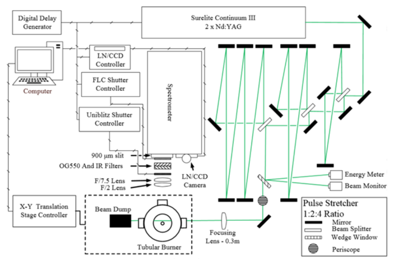
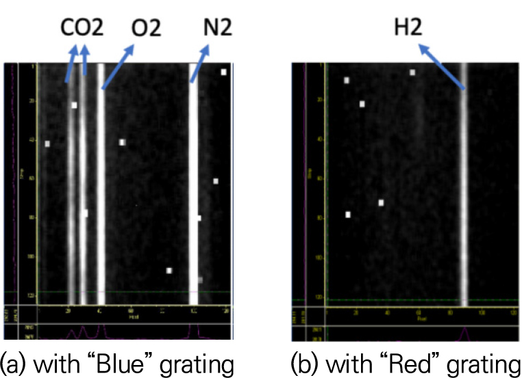
Two images with different grating angles of the modified 0.75 m Spex spectrometer were captured sequentially and combined to make the full spectrum from 561.20 nm to 698.71 nm per linear scan; the former is for spectral range of 561.20∼617.97 nm and the latter for 642.50∼698.71 nm. The spectrometer has a final dispersion of 0.39 mm/nm. Fig. 5 shows typical Raman spectra of cold air mixed with CO2 and H2, which were taken with “Blue” and “Red” grating angles of the spectrometer. Raster scans of linear measurement of a flame formed a two-dimensional data set of approximately 5 mm in length and 0.2 mm wide (dictated by the beam size). Resolution of measurements were determined as 86 μm × 200 μm as verified with a Ronchi grating and set by the translational stage of the burner.
In addition, chemiluminescence images of OH* and CO2* taken using a PI-MAX 4 (1024 × 1024) ICCD camera with an UG 11 filter were used to align the measurement origin to the desired region of interest; a sample image of the flame is to be discussed in the following chapter.
3. Calibration of Raman Signal
For the hydrogen-CO2-air flames, the calibration matrix Kij in Eq. (2) can be simplified for the five major species of CO2, O2, N2, H2O, and H2, based on theoretical Raman spectra simulated with RAMSES [20], as below:
The diagonal elements (or factors) of the calibration matrix are most significant and relate the Raman signal to the species number density while the off-diagonal ones relate the cross-talk of the different species on the others; for example, KCO2,O2 is the interference of the O2 spectrum on the CO2 Raman signal. The non-zero elements of the calibration matrix, which are temperature-dependent, were determined over a temperature range between 300 K and 2200 K.
The calibration matrix Kij in Eq. (4) was determined from the collected Raman signal within a 12.5 mm diameter Hencken burner flame, the calculated temperature and five major species - CO2, O2, N2, H2O, and H2 - concentrations. The non-zero elements of the calibration matrix were determined through three different steps, designated by three flow groups of HotLean, HotRich, and HotLeanCO2, as shown in Table 2.
The three flow groups include the corresponding cold flow, that is, ColdAir, ColdAirH2, ColdAirCO2, respectively, as shown in Table 3. Most of diagonal elements, that is, KO2, KN2, and KH2O and an off-diagonal KCO2,O2 were determined with the data of HotLean group flames. All the last column elements, that is, four off-diagonal KCO2,H2, KO2,H2, KN2,H2, KH2O,H2, and a diagonal KH2 with the data of HotRich group flames; The remaining two non-zero elements, KCO2 and KO2,CO2 with the data of HotLeanCO2.
Table 2.
Three flow groups of calibration flames and related elements in the calibration matrix
| Flow group | Target elements in the calibration matrix |
| HotLean | KO2, KN2, KH2O, KCO2,O2 |
| HotRich | KCO2,H2, KO2,H2, KN2,H2, KH2O,H2, KH2 |
| HotLeanCO2 | KCO2, KO2,CO2 |
Table 3.
Experimental conditions for calibrating the Raman scattering system*
The Hencken burner is widely used for calibration of both laser diagnostic probes including Raman scattering technique and physical probes in combustion science. The surface-mixing Hencken burner produces a flame that is flat, uniform, steady, and nearly adiabatic under the correct flow conditions [25, 32].
In the experiment, a 12.5 mm diameter Hencken burner was placed at the tubular burner location in Fig. 4 in such a way that the optical conditions remained the same between calibration and tubular flame experiments. Adiabatic equilibrium is assumed at 15 mm downstream from the burner face, and the Raman signals were collected from the spot for each and every flame condition, which include cold conditions, as shown in Table 3.
The reason many different flames were used is that all the temperature-dependent calibration elements need to be determined for the above temperature range. Gas flow rates for reactants were controlled with mass flow controllers (Teledyne Hastings HFC-202/203), and co-flow rates were measured with flow meter (Teledyne Hastings HFM-201). Flow controllers and meters are accurate to 1% full scale and were verified by laminar flow elements.
At the same time, the composition and the temperature in the post-flame zone were calculated by using an adiabatic equilibrium program [26]. Fig. 6 shows calculated temperature and mole fractions of major species of calibration flames. Calculated mole fraction values of major species in Fig. 6(b) were used as values of Nj in Eq. (2).
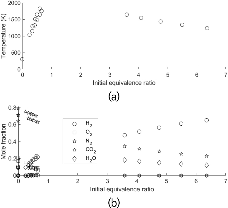
Fig. 7 shows Raman signal as a function of wavelength, ranging from 561.20 nm to 698.71 nm for all the calibration flames listed in three groups of Table 3 except three flames (Calibration_5, Calibration_10, & Calibration_15), one per each group due to the limitation of space.
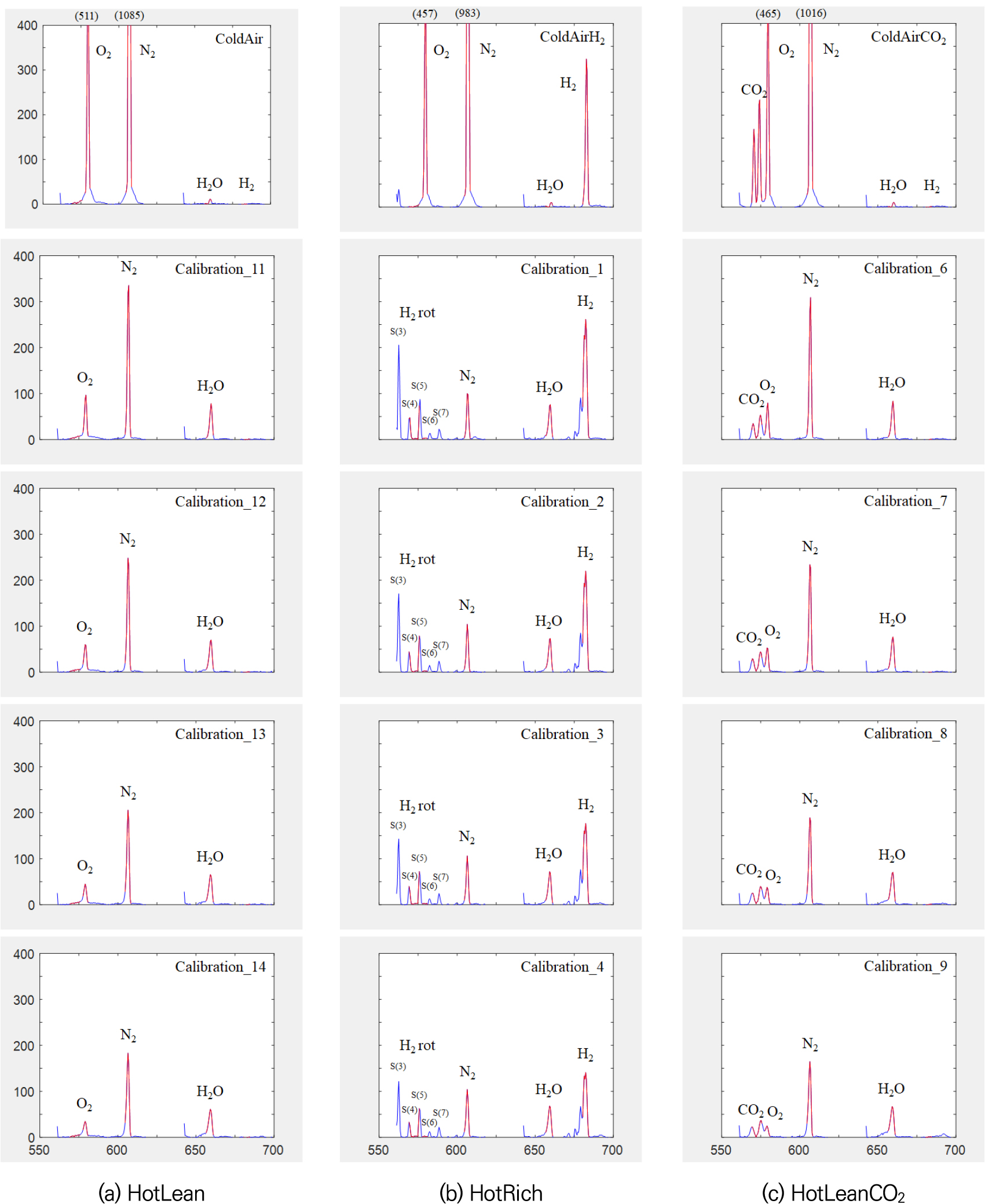
The red curves in Fig. 7 represent vibrational Raman signal intervals of the five species for the hydrogen-CO2-air flame occurring at wavelength (nm), CO2 (571.0, 574.4), O2 (580.0), N2 (607.3), H2O (660.5), and H2 (683.2). Note that the Raman signal designated as “H2 rot” in Fig. 7(b) and Fig. 12(a) represents H2 rotational Raman spectra, which is not used for H2 measurement. The top row of the figure show three cold images, that is, ColdAir (LHS), ColdAirH2 (CTR), and ColdAirCO2 (RHS), in Table 3. As expected, Raman signals of major species of each cold case can be seen clearly. The rest of the rows in the figure contain Raman images of each group as a function of initial equivalence ratio, as listed in Table 3. Eventually, Raman signals of all five species for each group as a function of temperature are available for the calibration of the Raman scattering technique. However, the order of magnitudes of Raman signals of all the species in the flames vary significantly, thus only signals exceeding the threshold values (species concentration: 1 × 10¹⁶ #/cm3) were used to calculate each calibration factor. The number of Raman data to be used for each calibration factor, ranging from 3 to 18, are different, depending on the size of the signals.
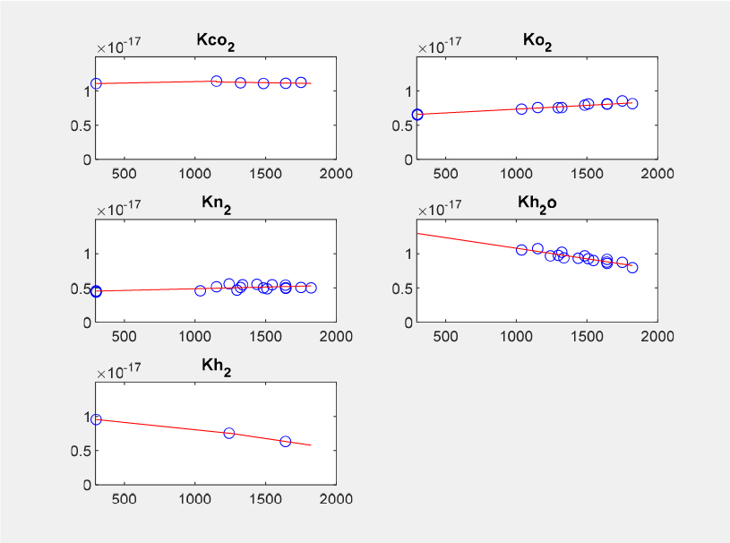
The calibration factors in Eq. (4), both main diagonal and off-diagonal elements, were obtained as polynomial functions of temperature. Due to the temperature dependence of calibration constant, the calibration factors have to be determined by finding local minimum of the object function using equations that include all the major species found in the flame, that is, CO2, O2, N2, H2O, and H2 by utilizing a MATLAB function of fminsearch. In this study, most of the polynomials were determined in either the 1st-degree or 2nd-degree, as shown in Figs. 8 and 9. The former figure shows the results for the main diagonal elements while the latter those for the off-diagonal elements. However, the degree of polynomials can be higher [33]. It is also noted that piecewise interpolation was used in some cases, for example, KCO2 and KH2.
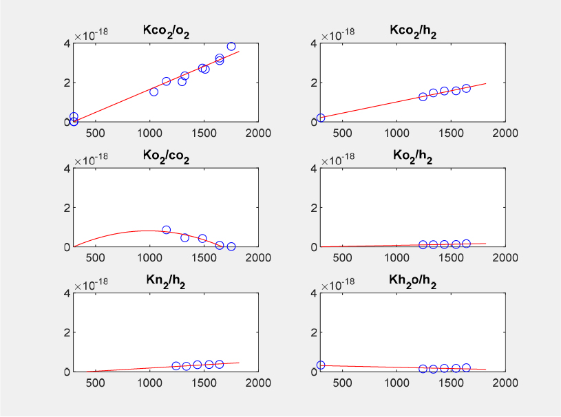
The polynomial coefficients for eleven non-zero elements in calibration matrix in Eq. (4) or calibration factors were determined and saved in cell MATLAB format during the calibration procedure, and will be used to calculate the temperature and the main species concentrations of a H2-CO2-air partially-premixed cellular tubular flames to be discussed in the following chapter.
4. A Hydrogen-CO2-Air Partially Premixed Cellular Tubular Flame
Temperature and major species profiles of the H2-CO2- air partially premixed cellular tubular flames were measured using the spontaneous Raman spectroscopy technique on a tubular burner at Vanderbilt University [27]. As shown in Fig. 3, premixed H2-air enters radially from the outer nozzle and impinges on a CO2-H2 mixture exiting a 6.35 mm diameter inner nozzle. The inner nozzle composition is 14% H2 and 86% CO2 by mole fraction with a velocity of 15.9 cm/s, which forms a weak cellular diffusion flames across moderate stretch rate κ. A wide variety of flame structures (axial view), that is, cellular, non-cellular, non- cellular with single cell, non-cellular with split-cell, can be created by varying the equivalence ratio from the outer nozzle [27].
A partially premixed tubular flame was investigated in this study, which is a non-cellular with (12-fold) single cell, in shown in Fig. 10 from [27]. The figure is (axial- view) chemiluminescence image of the flame, recorded from the bottom of the tubular burner. The image also shows the scanning region within the solid lined box. Note that the dashed-line circle in the figure represents the inner nozzle. Scans are taken linearly from bottom to top by 28 steps with the laser beam incoming from right to left, as shown in Fig. 11. The size of the interrogation region (x, y) is approximately 5.20 × 5.40 mm2. As previously explained in Section 2.2, the raster scans, dictated by the beam size, are of 0.2 mm wide.
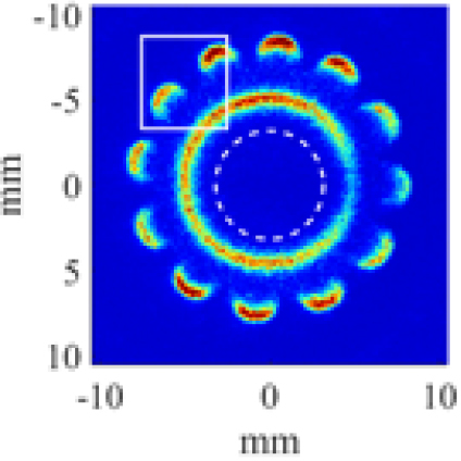
Fig. 10.
Cross-sectional (axial) view of a H2-CO2-air partially premixed cellular tubular flame for κ=130 s-1 with the outer nozzle of H2/air premixed reactants (ϕ=0.272) vs. the inner nozzle of diluted fuel (CO2:H2=6:1). The sold lined box represents the scanning region [27].
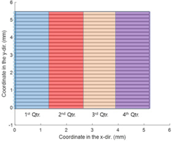
Fig. 12 shows representative Raman signals of the H2-CO2-air partially premixed tubular flame with both “Blue” and “Red” gratings at y = 2.0 mm for the grid shown in Fig. 11. The signals are a function of wavelength of the two gratings and imply mean values of each quarter of them in the x-direction, colored in Fig. 11 for clarity.
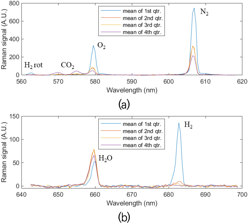
Fig. 12.
Representative Raman signal of the H2-CO2-air partially premixed cellular tubular flame with both (a) “Blue” and (b) “Red” gratings. The signal is a function of wavelength of the two gratings and the curves represent mean value of each quarter of them in the x-direction at y=2.0 mm of Fig. 11.
This variation in Raman signals along the x-direction will result in the change in temperature and species concentration of the flame to be explained shortly. Similar to the calibration Raman images, the resulting Raman images (file size: 124 × 123 × 56) were taken by LN cooled ICCD camera and further cosmic ray-cleaned, background- corrected, and energy-normalized.
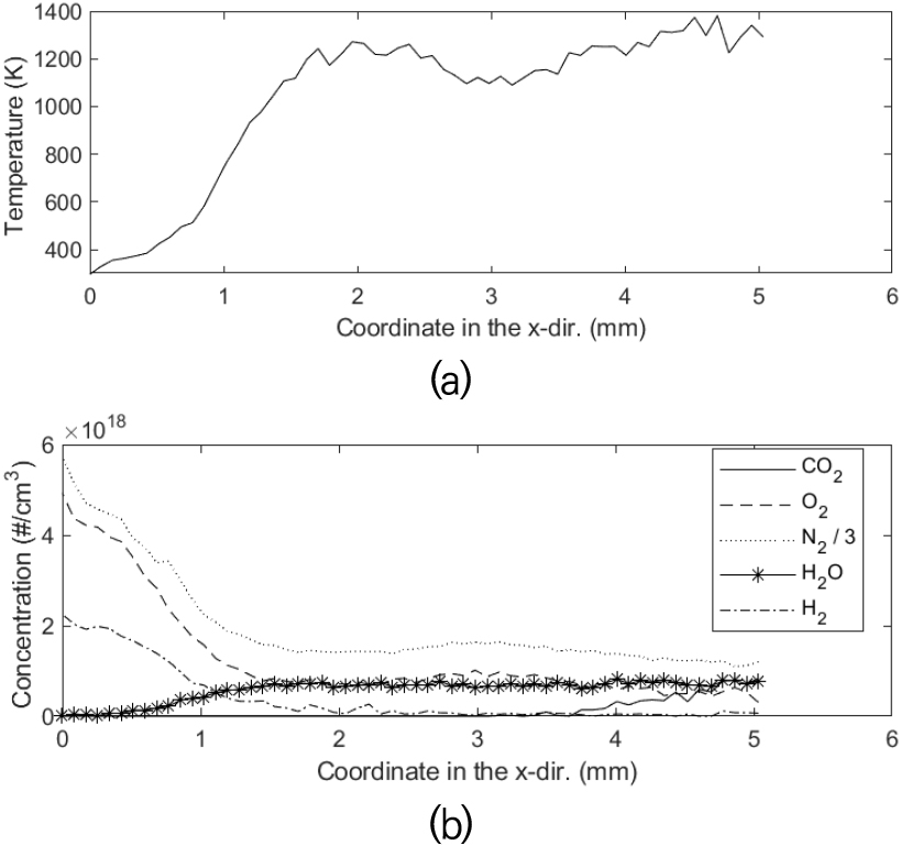
Along with the polynomial coefficients in calibration matrix found in the previous chapter, these Raman signals of 28 raster scans were used to determine major species concentrations and the temperature, based on Eqs. (2) and (3). Fig. 13 shows the variation of the calculated temperature and the major species concentrations in the H2-CO2-air partially premixed cellular tubular flame(ϕ=0.272, κ=130 s-1) along x-axis, representatively at y=2.0 mm. Uncertainty analysis of experimental errors of Raman measurements provided characteristics values for temperature uncertainty of approximately ±70 K for hot products and ±3 K for room temperature reactants. It also turned out the characteristic uncertainties for chemical species were approximately ±2% by mole fraction for hot products and ±0.5% for room temperature reactants.
In order to see two-dimensional structure of the flame, three-dimensional surface plots were performed, as shown in Fig. 14. The figure shows two-dimensional distributions of the temperature and five species concentrations in the interrogation area (5.20 × 5.40 mm2) in Fig. 10. In addition to this figure, radial profiles of the mixture fractions, mole fraction, local equivalence ratio, etc. can be plotted [27] and the whole structure of the flame can be reconstructed for further analysis.
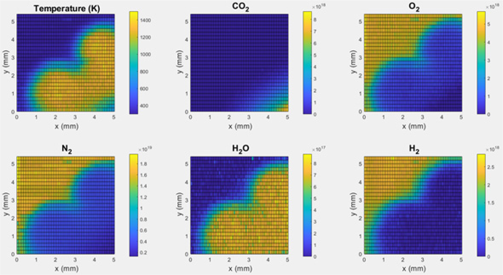
Fig. 14.
Spatially resolved Raman scattering measurements of the temperature and major species concentrations in the H2-CO2-air partially premixed cellular tubular flame for κ=130 s-1 with the outer nozzle of H2/air premixed reactants (ϕ=0.272) vs. the inner nozzle of diluted fuel (CO2:H2=6:1) [33].
5. Conclusion
A technical approach including data reduction of the Raman scattering technique for measurements of major species - CO2, O2, N2, H2O, and H2 - concentrations and temperature in hydrogen-CO2-air tubular flames, based on MI method, has been reviewed and modified by utilizing existing experimental data [33] and related MATLAB scripts. Most of Raman scattering data have been borrowed [33], although some experimental Raman data were collected in this work. Existing MATLAB scripts for preparing for the tubular flame experiments, calibrating Raman signals, reducing Raman spectra data, and finally plotting the results have been modified in some cases. The Raman spectra data were successfully reduced to investigate the structure of the tubular flame, generating maps of major species concentrations and temperature. A calibration method for the technique has also worked properly. It turned out that the technical procedure for Raman scattering technique investigated in this study works quite well. The approach described here for hydrogen/air tubular flame may be adapted to hydrocarbon/air tubular flames when other necessary species, for example, CH4 and CO for methane/air flame [34], are considered in the entire process.
