


1. Introduction
2. Experimental method
2.1 Principle of BOS
2.2 Experimental setup
2.3 BOS setup
2.4 Experimental conditions
3. Results and Discussion
3.1 Reconstruction of Two-Dimensional Flame Temperature Fields
3.2 Validation of BOS Reconstructed Radial Temperature Profiles
3.3 Time-Sequential BOS Temperature Reconstruction
4. Conclusion
1. Introduction
Density and temperature distributions are fundamental parameters for characterizing fluid-flow behavior. In combustion systems, temperature distribution reflects heat- release processes and flame structure, whereas density variations influence refractive-index changes that affect the propagation of light through the flow field[1]. Because combustion is still widely employed in energy-conversion and engine applications, accurate determination of these parameters is important for improving efficiency and reducing pollutant emissions[2,3,4,5,6].
Methods for measuring temperature and density can be classified as intrusive or non-intrusive. Thermocouples are widely used because they are simple, reliable, and suitable for direct temperature measurement at specific locations; however, they provide only local information and cannot capture the entire thermal field[7]. To overcome this limitation, optical techniques such as schlieren photography, interferometry, shadowgraphy, and near-field optical density measurements are employed to visualize refractive-index variations associated with density gradients in the flow[8,9]. However, many laser-based measurement systems require expensive instrumentation and complex optical alignment.
Background-oriented schlieren (BOS) is a non-intrusive optical technique for visualizing and quantifying density- gradient fields[10,11]. Compared with conventional schlieren, shadowgraphy, and interferometry, BOS uses a simpler setup consisting mainly of a camera, patterned background, and image-processing software[12,13]. Its large field-of-view capability and successful use in flow-visualization and density-measurement applications, including shock-wave studies, make it well suited for combustion diagnostics[14].
Previous BOS studies have shown its capability to reconstruct density and temperature fields in combustion flows, with accuracy mainly governed by image quality, experimental configuration, and displacement estimation [15]. Because these displacement fields are used to infer density and temperature, reliable image-processing tools such as PIVlab are commonly employed[16]. For axisymmetric BOS, inversion algorithms, Poisson-equation- based reconstruction, and Fourier–Hankel methods have been investigated to improve refractive-index-field accuracy and robustness[17,18]. Recent studies have further applied BOS to premixed-flame temperature reconstruction using thermocouple and chemiluminescence validation, while propane jet combustion studies have supported a broader understanding of combustion-flow behavior [19,20].
Despite these advances, BOS-based flame-temperature reconstruction remains sensitive to displacement estimation, optical calibration, and reconstruction assumptions. In combustion environments, steep temperature gradients, weak signals, spatial-resolution limits, and Abel-inversion sensitivity can affect accuracy. Therefore, practical validation of an accessible PIVlab-based BOS workflow remains valuable for small laboratory-scale propane–air flames under varying equivalence ratios.
In this study, a PIVlab-based BOS workflow is used to reconstruct two-dimensional temperature fields and radial profiles of axisymmetric premixed propane–air flames. The results are validated against corrected thermocouple measurements at y = 30 mm. The objective is to assess BOS performance under lean, stoichiometric, and rich conditions, including a representative time-sequential case for the stoichiometric flame.
2. Experimental method
2.1 Principle of BOS
The BOS method measures light-ray deflection caused by the refractive-index variation in a non-uniform density field. As shown in Fig. 1, light passing through the flame is deflected, producing image displacements and , which were used to determine the deflection angles, and . The corresponding displacement on the background plane is , where L is the calibration coefficient between the CMOS camera and the background. A total of 3000 flame-distorted images were compared with reference images and processed in PIVlab to obtain the average displacement field. Images were processed using multi-pass cross-correlation with 50% overlap, Gaussian sub-pixel peak fitting, and vector validation[16].
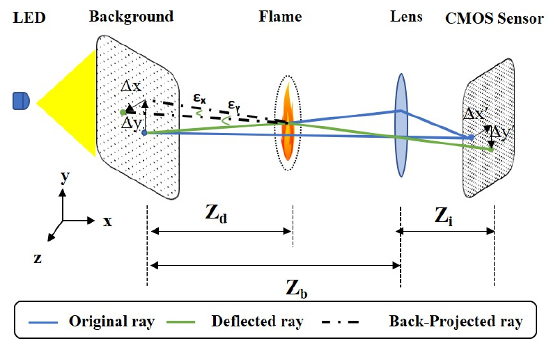
The pixel displacements were converted into the physical displacements using the checkerboard calibration. Under the paraxial assumption, the ray deflection angle is given by[19]:
where is the flame-center to background distance. The standard Abel transform was subsequently applied to Equation (1).
where r is the radial coordinate. The resulting inverse Abel transform can be expressed as follows:
Flame density was obtained from Eq. (4) using direct reconstruction[17,19]. The midpoint of the calibrated transverse domain defined the flame centerline and radial origin. Referencing the measured deflection field to this origin reduced errors from centerline offset and optical misalignment, although Abel reconstruction remains sensitive near the axis[17,18]. The refractive-index field was converted to density using the Gladstone–Dale relation. The coefficient and molecular weight were assumed to remain approximately constant between the premixed and fully reacted propane–air gases. This assumption is supported by previous studies on propane–air combustion systems, which report that the Gladstone–Dale coefficient varies only slightly due to strong nitrogen dilution in the combustion products. However, changes in equivalence ratio and reaction progress may still introduce small uncertainties, particularly in lean and rich conditions. Finally, the temperature was calculated using the ideal gas relation, where is the universal gas constant[20].
To assess the practical accuracy of the PIVlab-based BOS reconstruction workflow, mean absolute error (MAE) and root mean square error (RMSE) were calculated between the BOS-reconstructed radial temperature profiles and the corrected thermocouple measurements.
2.2 Experimental setup
Fig. 2 shows the experimental setup, including the high-speed camera, lens, speckled background, burner, laptop, camera-background stand, and propane-air supply system. The propane-air flame was generated using a circular premixed burner with an outlet diameter of 8 mm.
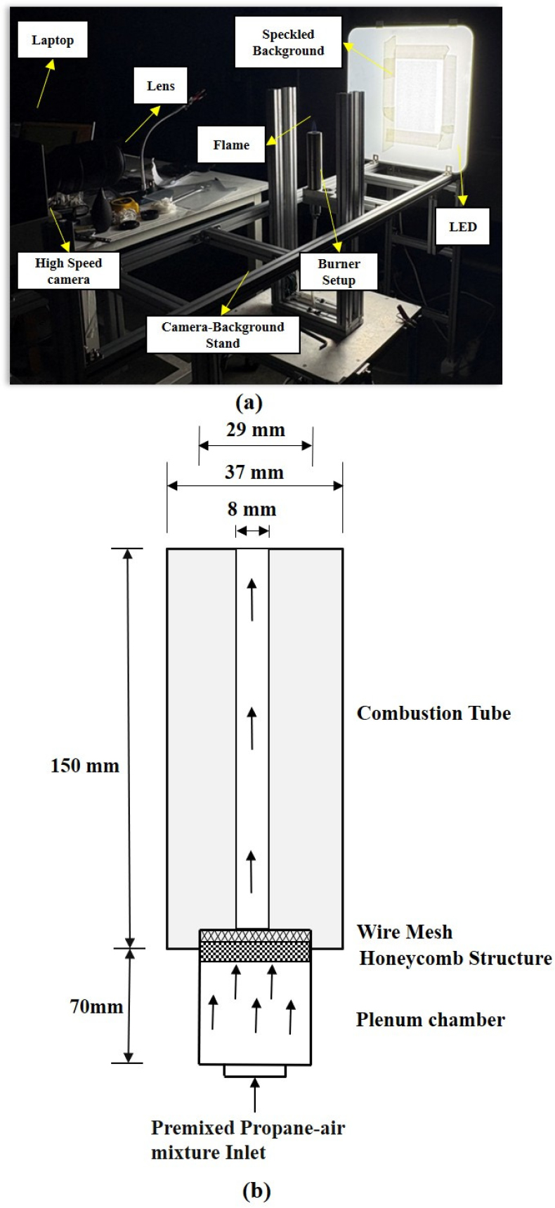
Propane and air flow rates were controlled using the mass flow controllers (ATOVAC, AFC500). The propane and air were premixed in a mixing chamber and passed through a honeycomb mesh before reaching the combustion tube. The honeycomb mesh was employed to straighten the flow and improve the uniformity of the premixed gas flow as shown in Fig. 2 (b). Under ambient conditions, the propane and air flow rates corresponding to each operating condition are presented in the experimental conditions section. The Reynolds number was determined from the burner outlet diameter and the unburned premixed-gas properties, according to , where is the bulk velocity. For the three equivalence ratio conditions, the Reynolds numbers were estimated to be approximately 9.21×10² to 9.33×10², indicating that the premixed flow at the burner exit was laminar for all operating conditions.
2.3 BOS setup
A MATLAB-generated BOS speckled target contained approximately 147,000 dots, with a projected dot size of about 2–3 pixels. The flame-background and camera-lens distances were selected to balance BOS sensitivity and spatial resolution. The camera was fixed and focused on the background so that flame-induced density gradients produced measurable dot-pattern displacements through light deflection. The flame-background distance was kept large enough to improve sensitivity but limited to reduce spatial-resolution loss. Reference and flame images were acquired using identical camera position, lens setting, and illumination conditions for reliable displacement calculation.
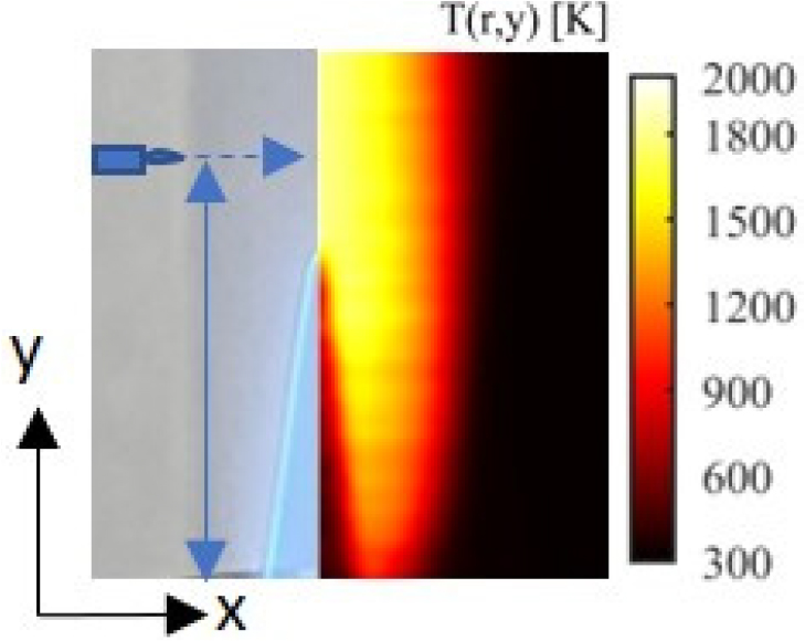
A cylindrical r-y coordinate system was defined with its origin at the burner-exit center, as shown in Fig. 3. Type B thermocouple measurements were taken at y = 30 mm at 2 mm radial intervals for validation. The measured thermocouple temperature was converted to kelvin and corrected for radiative heat loss using the steady-state bead energy balance , where and are the corrected gas, measured bead, and ambient temperatures, respectively.
For radiation correction, the thermocouple-bead emissivity was set to 𝜀=0.11, and the Stefan–Boltzmann constant was set to 𝜎=5.67×10⁻⁸W/(m2‧K4). The convective heat-transfer coefficient h was estimated from temperature-dependent gas properties using a Nusselt- number-based correlation. The bead diameter used in the correction was 2 mm. At y = 30 mm, the radiation correction ranged from approximately 0.57 to 75.75 K across all flame conditions. The corrected temperatures were used as reference data, and checkerboard calibration converted pixel displacement into physical displacement.
2.4 Experimental conditions
The detailed experimental conditions are listed in Table 1.
Table 1.
Experimental operating conditions
3. Results and Discussion
3.1 Reconstruction of Two-Dimensional Flame Temperature Fields
The BOS-reconstructed two-dimensional temperature fields of the stoichiometric, lean, and rich premixed flames are shown in Fig. 4. In all cases, BOS captures a central high-temperature region with a clear radial decay from the centerline toward the ambient region, indicating outward heat transfer. The stoichiometric flame shows the strongest and widest hot core, especially between y = 10-30 mm, consistent with higher heat release.
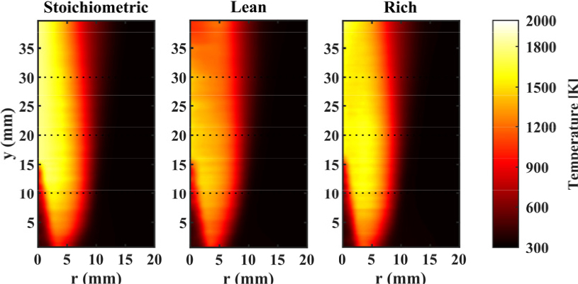
As shown in Fig. 4, the effect of equivalence ratio is interpreted by considering adiabatic flame-temperature trends, flame structure, and BOS spatial resolution. The lean flame shows a weaker thermal field because excess air lowers flame temperature and weakens refractive-index gradients, reducing the BOS response. The stoichiometric flame shows the strongest thermal field, consistent with conditions near the maximum adiabatic flame temperature. Under rich conditions, a compact high-temperature region appears near the centerline due to changes in flame structure associated with limited oxidizer availability and incomplete combustion. Thus, the reconstructed differences reflect both combustion behavior and measurement limitations. Near the burner exit, the thermal field is still developing, while above y = 30 mm, elevated temperatures remain near the centerline, particularly for the stoichiometric and rich flames.
After reconstructing the two-dimensional temperature fields, radial temperature profiles were extracted at several axial heights to evaluate the BOS reconstruction trend. As shown in Fig. 5, all cases exhibit a clear temperature decrease from the flame core toward the ambient region. At lower heights, the sharp radial decay to below 900 K indicates that BOS captures regions with strong thermal gradients. At y = 20 mm, the central temperature increases in all cases, reflecting the development of the high- temperature reaction zone. The stoichiometric flame reaches the highest temperature, whereas the lean flame shows the lowest because of dilution by excess air.
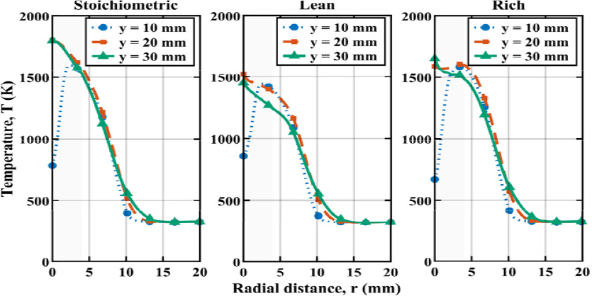
The rich flame remains between these two cases due to incomplete combustion. At y = 10 mm, the drop in radial temperature becomes more pronounced. In the stoichiometric case, the temperature decreases to around 800 K away from the centerline. Although the lean flame generally shows the lowest reconstructed temperature, a slightly higher central temperature appears locally at y = 10 mm, which may be linked to local flame fluctuations or sensitivity of the reconstruction method. The rich case shows a sharp decrease, approaching 600 K in the outer region. These variations suggest higher sensitivity and uncertainty near the lower flame region. At higher axial locations, the expected trend becomes clearer, with stoichiometric having the highest temperature, followed by the rich and lean cases.
Overall, the results show that BOS captures radial temperature decay, consistent with radial trends, and distinguishes the thermal behavior at different equivalence ratios, supporting its use as a non-intrusive flame-temperature measurement technique.
3.2 Validation of BOS Reconstructed Radial Temperature Profiles
After analyzing the two-dimensional BOS temperature fields, radial temperature profiles were extracted at y = 30 mm and compared with thermocouple measurements, as presented in Fig. 6. This location was chosen because the reconstructed temperature fields showed a well-developed hot core and clear radial temperature gradients between the inner flame zone and the surrounding ambient region, making it suitable for comparison with thermocouple measurements.
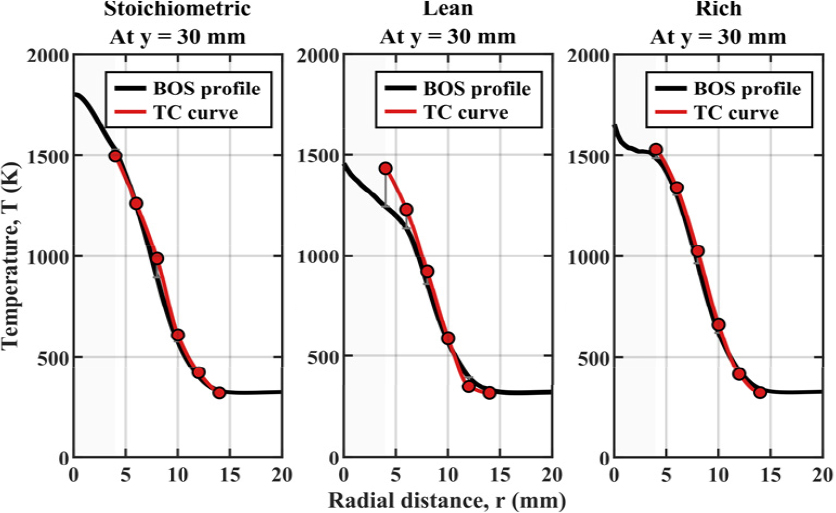
For all equivalence-ratio conditions, the BOS results reasonably reproduced radial temperature behavior, with the temperature decreasing from the flame core toward the outer radial region. For the stoichiometric and rich flames, the BOS-reconstructed profiles show good agreement with the thermocouple data over most of the radial domain. This agreement is also supported by the error values listed in Table 2, where the stoichiometric and rich cases have MAE values of 33.19 K and 35.86 K, and RMSE values of 44.28 K and 38.75 K, respectively. In contrast, the lean flame shows larger errors, with MAE and RMSE values of 70.08 K and 91.67 K, respectively. This may result from its weaker temperature field, which produces smaller refractive-index gradients and reduces the BOS displacement signal. Since thermocouple validation was limited to y = 30 mm, additional axial validation, repeated measurements, and error-bar analysis are required in future work.
Table 2.
MAE and RMSE for BOS-TC temperature validation at y = 30 mm
| Flame conditions | MAE (K) | RMSE (K) |
| Stoichiometric | 33.19 | 44.28 |
| Lean | 70.08 | 91.67 |
| Rich | 35.86 | 38.75 |
The error metrics in Table 2 indicate that displacement uncertainty, limited spatial resolution, and Abel inversion sensitivity affect the reconstructed temperature profiles. The higher RMSE than MAE suggests that discrepancies are concentrated near the hot core and regions with steep temperature gradients rather than being uniformly distributed. Under weaker gradient conditions, reduced optical sensitivity may also produce smaller BOS displacement signals.
Uncertainty arises from displacement estimation, optical calibration, centerline detection, Abel inversion, and thermocouple correction. PIVlab results may be influenced by background-dot quality, image noise, interrogation-window size, and sub-pixel interpolation. Calibration errors affect the conversion of pixel displacement into physical displacement, while small centerline errors become significant near r = 0, where Abel inversion is most sensitive.
Thermocouple measurements introduce additional uncertainty due to the approximately 2 mm bead size, spatial averaging, radiation correction, probe positioning, and possible flow disturbance. Therefore, the MAE and RMSE values represent combined BOS–thermocouple discrepancies rather than BOS uncertainty alone. Nevertheless, the maximum RMSE remained below approximately 92 K, indicating that BOS reasonably captured the radial temperature distribution, although accuracy varied with flame conditions.
3.3 Time-Sequential BOS Temperature Reconstruction
To examine the sequential BOS reconstruction capability, 500 consecutive images of the stoichiometric premixed flame were processed, and four representative temperature fields at selected time instants are presented in Fig. 7. The contours at t = 0.000, 0.167, 0.333, and 0.500 s indicate that the high-temperature region is mainly concentrated near the inner flame core and gradually decreases toward the surrounding ambient region.
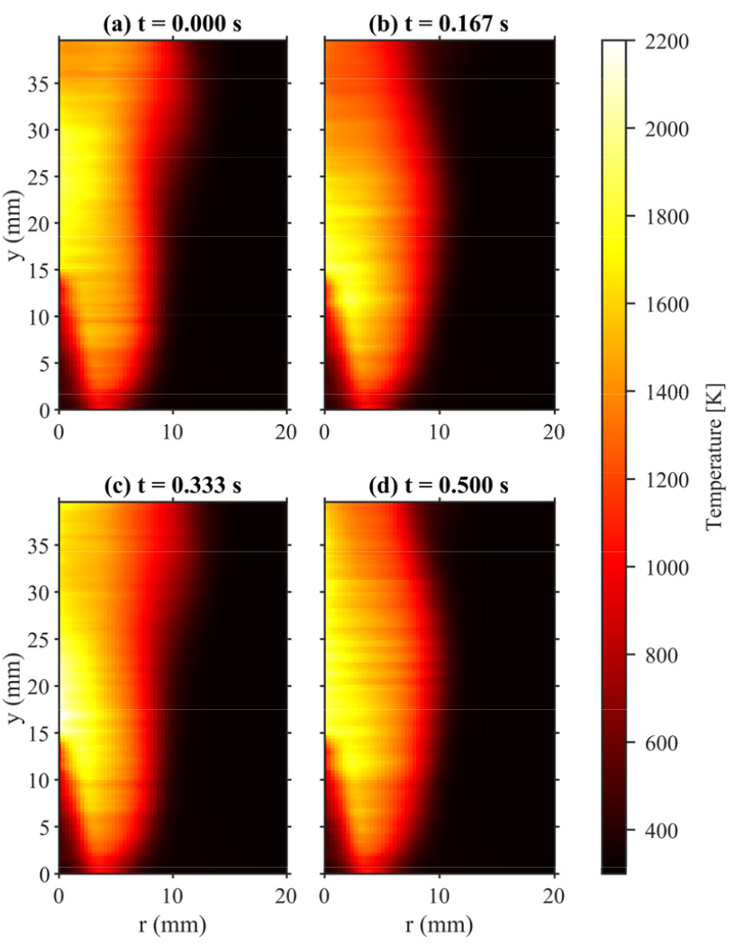
Noticeable but moderate variations between frames can be observed in the size, intensity, and radial extent of the hot core, which may be attributed to inherent flame unsteadiness as well as measurement uncertainty. The four fields shown in Fig. 7 are representative snapshots selected from the 500 reconstructed images and are not intended to provide a quantitative assessment of flame stability. Instead, they suggest that the overall spatial structure of the reconstructed temperature field remains broadly consistent over the 0.5 s observation period. A rigorous evaluation of temporal stability would require a time-resolved statistical analysis of parameters such as peak temperature, hot- region area, and temperature fluctuations, including their standard deviations.
4. Conclusion
This study applied the background-oriented schlieren (BOS) technique to reconstruct temperature profiles of premixed propane-air flames under lean, stoichiometric, and rich conditions. The results showed reasonable agreement with thermocouple data at y = 30 mm. The key findings are summarized below.
1)BOS reasonably captured the main temperature-field structure for all cases. The stoichiometric flame exhibited the strongest and widest high-temperature region, while the lean flame showed lower intensity and the rich flame displayed a more localized hot core.
2)Quantitative comparison indicated that the stoichiometric and rich cases showed better agreement with thermocouple data. The stoichiometric case had an MAE of 33.19 K and an RMSE of 44.28 K, while the rich case had an MAE of 35.86 K and an RMSE of 38.75 K. In contrast, the lean case showed the largest deviation, with an MAE of 70.08 K and an RMSE of 91.67 K, likely due to weaker refractive-index gradients, lower displacement signals, and inversion sensitivity.
3)The observed errors include combined BOS-thermocouple discrepancies and additional uncertainty from thermocouple-related effects such as probe positioning, spatial averaging, and flow disturbance.
4)Sequential BOS reconstruction of the stoichiometric flame showed that the dominant temperature-field structure was generally maintained over the 0.5 s observation period. This result indicates the potential of BOS for time-sequential temperature-field observation, although further quantitative temporal analysis is required.
Overall, BOS is a promising non-intrusive method for flame-temperature reconstruction, although repeated measurements, improved centerline validation, additional axial validation, and uncertainty quantification are needed.